Fully-Arbitrary Learned Color Filter Mosaics

Fully-Arbitrary Learned Color Filter Mosaics

This article presents a machine-learning method for demosaicing images, in which the mosaic itself and the demosaicing network are jointly optimized without any constraints on the mosaic pattern.  The system is capable of learning any color filter mosaic, up to and including a unique color filter on every pixel.  Code is available on Github: https://github.com/evanfletcher42/DeepMosaic

---

I recently read two papers on using convolutional neural networks for image demosaicing.  One focused on de-bayering and denoising images under a Bayer pattern (Gharbi et al, 2016); the other very recently extended this work to  color filter arrays (Syu et al, 2018) that are learned jointly with the demosaicing network.

One concern I saw with both architectures – especially the learned-mosaic extension in (Syu et al, 2018) – is that the nature of the color filter is tightly coupled with manually-specified parameters in the network architecture.  (Syu et al, 2018) learns a repeating color filter patch – 3×3 in their examples – the measurements under which, like (Gharbi et al, 2016), are then separated onto a number of color planes equal to the number of unique filters in the color filter array.

The primary worry is that these decisions apply arbitrary limits to the color filter arrays that can be learned.  Explicitly choosing an array of repeating 3×3 patches means the system cannot learn many possible mosaic patterns, including the industry-standard 2×2-repeating Bayer pattern, or any other arrangement that does not repeat with a period of 3.  Additionally, placing data from under every unique color filter onto separate color channels (9 channels for the 3×3 example) puts a practical limit on how many unique colors can be learned; since every additional color filter adds a channel to the network input, the amount of data and compute required can quickly become untenable.

In this post, I present a method which is capable of learning fully-arbitrary color filter arrays, with no constraints on arrangement or number of unique filters – it’s capable of learning a unique color filter on every pixel of the simulated image sensor, and pays no computational penalty for doing so.

Network Architecture

The network in this approach consists of:

1. The simulated mosaic layer, which contains the color filter array as trainable weights, and embeds the simulated mosaiced image and the mosaic itself into a fixed 3-channel representation.  (More on this later.)
2. A first layer of 64 3×3 convolutional filters
3. N repeating blocks of:
   • 64 3×3 convolutional filters;
   • A batch normalization layer;
   • A SELU activation layer;
   • An “add” layer in the style of ResNet, acting as a skip connection over this block.
4. A final 1 x 1 convolutional layer reducing the number of channels to 3 for the output RGB image.

The architecture is inspired by (Syu et al, 2018), except there is no explicit skip connection that avoids the entire CNN.

The network contains a total of 113,923 trainable parameters.  A residual structure, plus batch normalization and SELU activation, is employed to accelerate training.  Implementation is in Python, using Keras with the Tensorflow backend.  Batch size was 35 images; training ran for 100 epochs (~24 hours on a NVIDIA GTX 970).

In a way, this architecture is similar to an autoencoder: The mosaic layer creates an “encoded” representation with reduced dimensionality – the intensities that would be detected on an image sensor behind the color filter array – then learns a convolutional decoder to recover the original input image.

Mosaic Layer & CFA Embedding

A custom Keras layer is implemented to simulate the image sensor and embed information about the color filter array.  The key code for this layer is as follows:

def call(self, x):
    dot_product = K.sum(x * self.cfa, axis=3, keepdims=True)
    cfa_contrib = dot_product * self.cfa
    return cfa_contrib

First, we perform a per-pixel dot product between the RGB input and the weights in the layer that represent the color filter array, producing a monochrome image representing the intensities measured on an image sensor.  This acts as an approximation of how a color filter would attenuate certain wavelengths and pass others, and from an information standpoint, causes the network to lose the full RGB information from the input pixels.

Second, we take the weights representing the color filter and multiply them, per pixel, by the monochrome image from the first step, producing a 3-channel output image.   This is the key innovation – by doing this, we embed information about a potentially per-pixel-unique color filter array in a differentiable fixed-size representation.

From an information standpoint, the nature of the color filter on each pixel in a physical implementation is fixed and would be known; this is simply a scaling of that known information by a 1-channel quantity that would be measured by an image sensor.

Dataset & Training

Training and validation data is generated from the Flickr500 dataset, presented in (Syu et al, 2018).  This dataset contains a wide variety of images which have been downsampled from their original capture resolutions, so that any artifacts of the original bayer patterns in the cameras used for capture would not be present in the dataset.  Patches equal in size to the target mosaic are randomly selected from all training images.

Given that this network seeks to learn a fully-arbitrary color filter array over a relatively large image patch, the dataset must be designed so as to avoid overfitting to any local feature or geometry in the training set.  To this end, for each selected patch location, every possible patch containing this location is added to the training set.  For a 16 x 16 target mosaic size, 256 images will be considered for a single source location.

Including augmentation, the training set contains 2,048,000 image patches generated from 490 images; this number could easily be increased with strategies to page batches in and out of RAM.  Validation is performed on 10,240 patches, generated from 10 images kept separate from the training set.

Results

After training for ~24 hours, the learned color filter array looks quite familiar:

The network seems to have learned something very similar to a RGGB Bayer pattern, complete with 2×2 repetition and the pentile arrangement of the green pixels!  This was quite surprising, especially given that there is no spatial constraint on arrangement or repetition in this network design whatsoever.

This result is after 100 epochs – however the bayer-like pattern seems to arise very quickly, within the first epoch.  This video shows the color filter array weights during training, with each frame representing 100 batches:

In this video, the same bayer-like pattern appears to arise from two different points in the filter array, with a different phase; these then spread across the filter array, until they meet near the middle.  I speculate that a stalemate of sorts forms at that point, since the patterns on the left and right side of the image are very similar with the exception of a 1-pixel phase offset, and are likely “equally good” as far as demosaicing is concerned.  The precise location and shape of this “stalemate” zone seems highly sensitive to weight initialization and training data.

This potentially means the solution represents a local minimum; a uniformly-repeating pattern with no “stalemates” between phase offsets may be more optimal.  Strategies for breaking these “stalemates,” and allowing one phase offset to take over another, may be devised in the future.

It is worth noting that, while the learned color filter array strongly resembles a repeating Bayer pattern, each pixel in the CFA is technically unique – i.e. all of the green pixels are ever so slightly different from each other.  The grouping is so close that, for a practical implementation, it may be possible to select a reduced quantity of color filters for manufacture.

Analysis & Comparisons

The trained network is evaluated against three “traditional” (non-machine-learning) demosaicing approaches, mostly chosen because they were already implemented in the Python colour-demosaicing package:

1. Naive bilinear demosaicing
2. High-Quality Linear Interpolation for Demosaicing of Bayer-Patterned Color Images (Malvar et al, 2004)
3. Demosaicing with directional filtering and a posteriori decision (Menon et al, 2007)

 

I would have liked to include a comparison against the learned-mosaic method in (Syu et al, 2018); however, at the time this article was written, their code was not available (the link on the authors’ website stated that it was “coming soon”).

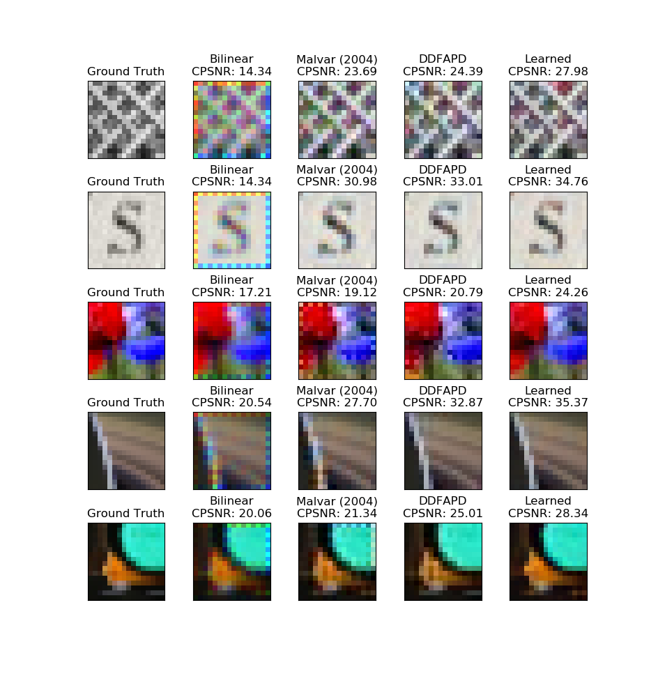
Test images were manually chosen from images separate from the training and validation sets; images were chosen to be generally challenging for demosaicing approaches, with high-contrast edges and small features.  The learned approach presented in this article yields a higher (CPSNR) than all other tested approaches on the test set.

Visualizing the convolutional filters via this method at the end of each residual block shows a few interesting patterns.  There are relatively few filters, so we can visualize all of them:

We can also visualize the input images which maximize the red, green, & blue channels at the output.  Not much is surprising here, aside from an abundance of green causing a peak activation for blue.

Conclusions

This optimization appears to have independently confirmed the venerable Bayer pattern as a good choice for a mosaic function – it was fascinating to see a familiar pattern arise from an unconstrained optimization.

There is the possibility of some inherent bias in the training dataset.  As the training images were captured using cameras that almost certainly use a Bayer pattern themselves, there is a concern that Bayer artifacts (i.e. reduced resolution in red/blue vs green) may be what is driving the Bayer pattern to arise in the learned color filter array, despite efforts to hide or reduce these Bayer artifacts in the training set.  I may try training with fully synthetic rendered data, which would never involve a Bayer pattern, in an effort to eliminate this possibility.

Approaches which explicitly limit the number of unique color filters do have practical advantages: they would be much more possible to fabricate, and the forced tiling should prevent local phase offsets from arising and persisting in the optimized pattern.  Given that the learned mosaic using this unconstrained approach is similar to a Bayer pattern with an apparent 2×2 repetition, it may be advantageous to explicitly force this repetition to accelerate training and possibly improve performance.

Bonus: Intentional Overfitting

For the approach presented in this article, care was taken that the chance of overfitting to local structure in the 2-million-image training set was minimized.

But what if we threw all of that out, and instead trained the network on exactly one image?

Training was quite fast, and produced a random-looking color filter array which does not look like a chicken (but, ostensibly, encodes one well):

When evaluating this massively overfit network, we see that it is capable of reproducing the training image almost exactly.  Other images, including palette swaps and an mirrored version of the training chicken… not so much.  In most cases, the output image is still visibly related to the structure of the input, if only slightly – and is typically a completely wrong color.  Curiously, it seems to like turning things red a lot.

Visualizing the convolutional filters shows that the network learned some structure, but not anything that directly looks like a chicken.  Well, maybe 1 or 2 of these kinda do, if you squint.  The lack of a strong color filter array is also apparent.

References

Syu, N. S., Chen, Y. S., & Chuang, Y. Y. (2018). Learning Deep Convolutional Networks for Demosaicing. arXiv preprint arXiv:1802.03769.

Gharbi, M., Chaurasia, G., Paris, S., & Durand, F. (2016). Deep joint demosaicking and denoising. ACM Transactions on Graphics (TOG), 35(6), 191.

He, K., Zhang, X., Ren, S., & Sun, J. (2016). Deep residual learning for image recognition. In Proceedings of the IEEE conference on computer vision and pattern recognition (pp. 770-778).

Klambauer, G., Unterthiner, T., Mayr, A., & Hochreiter, S. (2017). Self-normalizing neural networks. In Advances in Neural Information Processing Systems (pp. 971-980).

Ioffe, S., & Szegedy, C. (2015). Batch normalization: Accelerating deep network training by reducing internal covariate shift. arXiv preprint arXiv:1502.03167.

Malvar, H. S., He, L. W., & Cutler, R. (2004, May). High-quality linear interpolation for demosaicing of Bayer-patterned color images. In Acoustics, Speech, and Signal Processing, 2004. Proceedings.(ICASSP’04). IEEE International Conference on(Vol. 3, pp. iii-485). IEEE.

Menon, D., Andriani, S., & Calvagno, G. (2007). Demosaicing with directional filtering and a posteriori decision. IEEE Transactions on Image Processing, 16(1), 132-141.